The column angle shows the angle between the two polarizers.
The column correlation shows the correlation factor of the actual test results.
The column "++" shows the actual number of runs in which in both + detectors a photon is detected.
The column "+-" shows the actual number of runs in which in alice's + detectors and in bob's - detector a photon is detected. etc.
|
|
- The first line shows the results when the angle between both polarizers zero degrees is.
One possible actual result (of 10 tests) with an angle of zero could be:- + +, + +, - -, + +, - - , - -, - -, + +, - -, + +
- The result "+ +" means that in the two "+" detectors each a photon is detected. The result "- -" means the same for the "-" detector.
The table shows the results of 72 tests. In reality when you perform 1000 tests you could get something like: 498 "+ +" and 502 "- -"
The physical meaning is that the results are highly correlated.- line 9 shows the results when the angle between both polarizers 90 degrees is. One possible actual result (of 10 tests) with an angle of 90 degrees could be:
- + -, - +, - +, - +, + - , + -, - +, + -, - +, + -
- The result "+ -" means that in Alice's "+" detectors a photon is detected and in Bob's "-" detector also. The result "- +" means the reverse.
The physical meaning is that the results are highly anti-correlated. The correlation factor = -1- line 5 shows the results when the angle between both polarizers 45 degrees is. One possible actual result (of 10 tests) with an angle of 45 degrees could be:
- + +, - +, - -, - +, + - , + +, + -, - -, - +, - -
- What the results of the tests show that the probability for each of the 4 possible outcomes is the same. The physical meaning is that the results are completely random. The correlation factor = 0
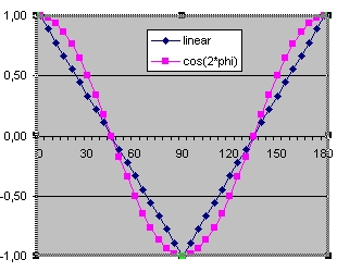
- In the "Graphical correlation", the blue line shows of the correlations calculated based on the simulated results of 36 runs. This are the same results as in the "Correlation table".
The pink curve shows the correlation function cos(2*phi). This correlation function describes the results predicted by the quantum theory.